
Essay · DIY Lab
Can you separate the drone from the bagpipe in a field recording?
We fed an algorithm a recording of a real piper from Teverga, nearly 50 years old, and tried to separate the drone from the melody before analyzing it. The standard technique for this, HPSS, is what we used in this small experiment — and here's the result, honestly.
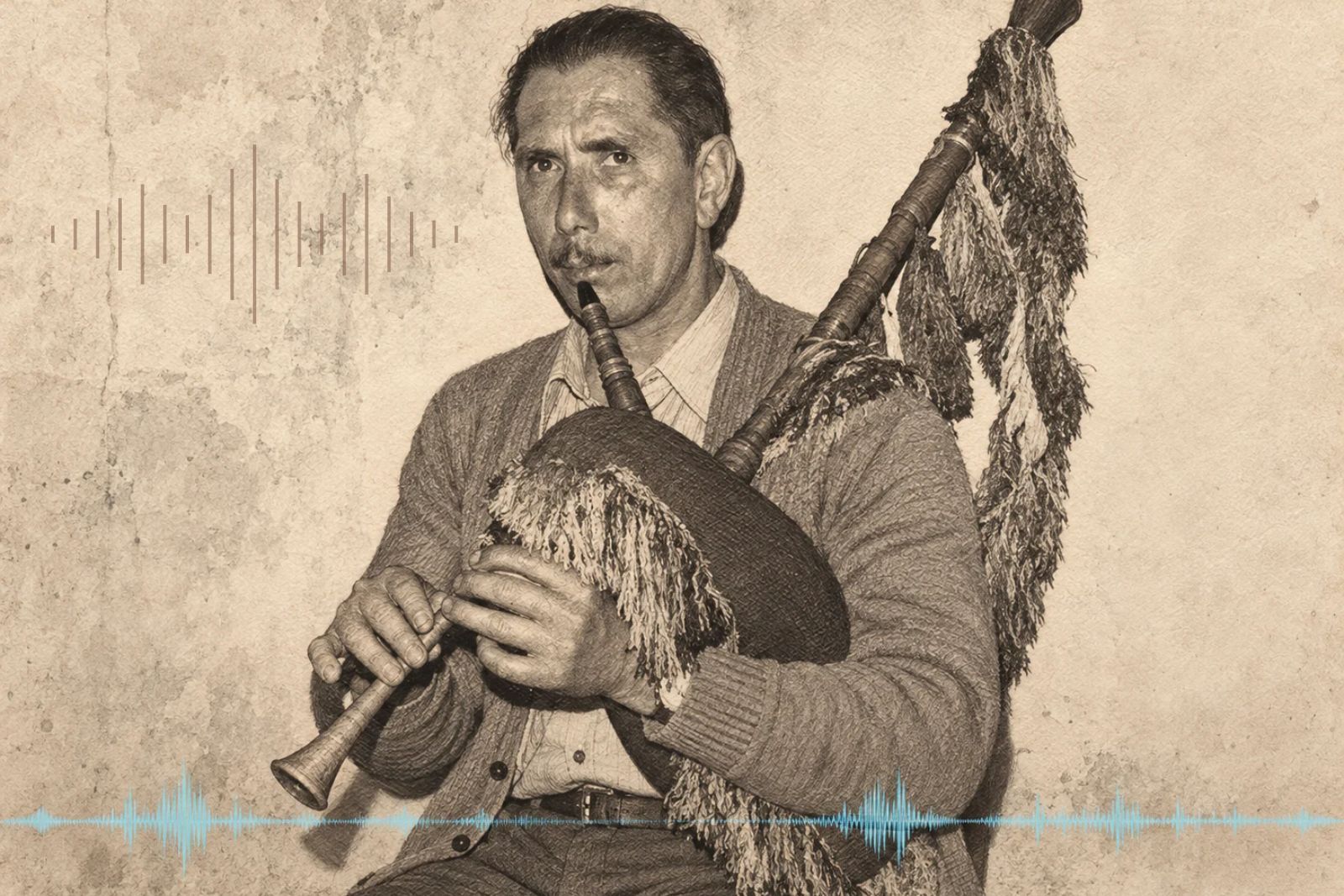
In April 1976, Celso Peyroux recorded Juan Huerta, a piper from La Torre (Teverga), on cassette tape playing the Asturian bagpipe. The tape is now part of Celso’s own Sound Archive, and the catalogue entry describes him this way: “one of the great pipers Teverga had, alongside Julio de Fresnedo and Floro Regina. They played for baile agarrao [a close-hold couple dance].” Almost fifty years later, I ran a fragment of that recording through an algorithm to try to answer a very specific question: can a program automatically separate the roncón (the continuous drone) from the melody of the punteru (chanter) — the two voices that sound at once in a bagpipe? And if it can, does that actually help us understand the music better?
The tool I use for this is called Music Information Retrieval (MIR): the branch of computer science that teaches a computer to “listen” to audio and extract information from it — when each note starts, what pitch it has, how loud it sounds. It isn’t magic or artificial intelligence in the sense of “understanding” music: these are algorithms that measure patterns in the sound wave.
This experiment is not a musical portrait of Juan Huerta, nor a piece of ethnomusicology — that human portrait of him lives on tever.es, in Gaiteros de la Tradición #4. Here I stay on technical ground, but told for anyone who has never looked at a spectrogram in their life.
Why the drone is the underlying problem
When an Asturian bagpipe sounds, you’re actually hearing two instruments mixed into a single sound, with no way to separate them by ear alone: the roncón (or drone), a pipe that produces a single fixed, continuous note throughout the whole piece — like a low hum in the background that never stops — and the punteru, the fingered pipe that plays the melody on top. Think of the roncón as the bass in a band that never stops playing the same note: there isn’t even a brief silence where you could “hear it alone” to learn what it sounds like in isolation. It’s always there, mixed in, all the time.
That’s a problem for any algorithm. If you want a program to analyze only the melody — only the punteru — it would first have to remove that constant hum of the roncón. And since there’s never a gap of silence to learn “this is just background noise” from, the algorithm starts out at a real disadvantage.
This article walks through the experiment in five steps:
- I check how good the recording itself is.
- I locate the roncón within the sound.
- I analyze the complete piece as it arrives, untouched.
- I try to separate the roncón from the melody.
- I compare whether that separation improved anything at all.
Before getting into the technical detail, here’s what gets analyzed: 19 seconds of that 1976 tape, as it sounds, unprocessed. Specifically, it’s the floréu d’entamu — the opening flourish — of an entemediu de misa: a short piece played during the pauses of a Mass.
What quality the recording has
This is a field tape recorded on cassette in 1976, not a studio take, and that shows up in the audio itself in measurable ways. To see it I use a spectrogram: an image that shows which frequencies (low, high) sound at each instant, like a kind of “X-ray” of the sound over time. In that image there’s a background noise very typical of old electrical equipment — mains hum — at 49.80 Hz, with a higher-pitched echo at 150.7 Hz that is almost exactly three times that frequency (150.7 divided by 49.80 gives 3.03, practically 3). That matches electrical mains noise, not anything musical: both tones sound with near-perfect stability — they barely vary from one instant to the next — and that absolute steadiness is precisely the signature of a background hum, not a note played by a person.
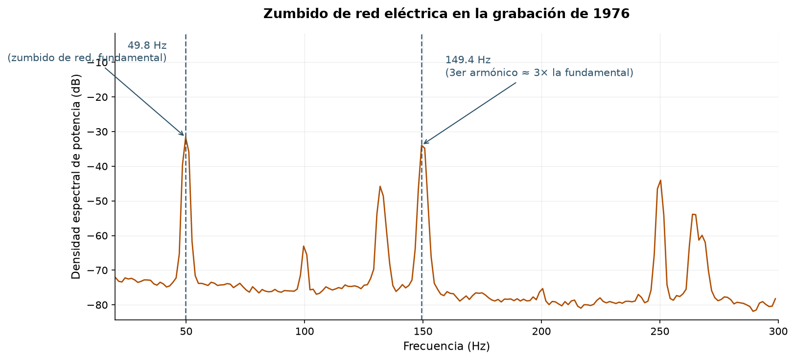
The two peaks of the mains electrical hum, almost three times higher in pitch one from the other: the unmistakable signature of an old device, not of anything musical.
As for how loud or quiet the recording sounds: I measure this with RMS, a standard way to calculate “how loud it sounds on average” for a signal (unlike the highest single peak, RMS summarizes sustained loudness). In decibels (dB, the unit we measure volume in: the more dB, the louder) that average fluctuates by 15.2 dB between the quietest and loudest moments of the full piece. An honest clarification is needed here: in an Asturian bagpipe recording there is no moment of real silence to measure, because the roncón sounds the whole time — so I can’t compare “signal against silence” to calculate how clean the recording is, as I could with a voice or a piano, which do pause between phrases. So instead I measure how much the volume of the full mix rises and falls: it’s the metric that actually makes sense when the “background” never stops sounding.
Where the drone lives within the sound
Before trying to separate it, I needed to confirm exactly which frequency the roncón lives at. To avoid confusing it with the mains hum from the previous section — a real trap, because its harmonics fall close to the roncón’s band — I relocated that hum with precision (49.80 Hz) and split the fragment into 18 one-second windows, checking in each one which frequency was the strongest and discarding any candidate too close to the hum’s harmonics. The real fundamental of the roncón is the frequency that wins most often across those 18 windows.
The result: 132.0 Hz, note C3, with 12 of the 18 windows voting for that value as the fundamental — a dominant, consistent result. To measure how far that tuning strays from the “official” one, musicians use cents: each semitone is divided into 100 equal parts, so a note at +15.6 cents is barely a sixth of a semitone above standard — a difference so small that almost no ear notices it. Relative to standard C3 in A440 tuning, that’s +15.6 cents: practically standard tuning, slightly sharp. That frequency appears prominently in 55.4% of the windows analyzed. Above the fundamental, the roncón also produces harmonics: higher-pitched echoes at exact multiples of the base frequency. Those harmonics vary more in intensity because they mix acoustically with the punteru melody sounding above them — only the roncón’s fundamental note holds that characteristic steadiness of a drone.
That the roncón sounds in C is no coincidence or free choice of the instrument: it’s the harmonic accompaniment the bagpipe carries when it plays alone or only with drum, and that’s why its note is always the punteru’s tonic — the note of rest, the one the melody resolves onto — but two octaves below the low C (C5) the punteru itself plays. Measuring 132 Hz and confirming it’s C3 isn’t just a tuning data point: it’s confirmation that this bagpipe is, in fact, tuned in C.
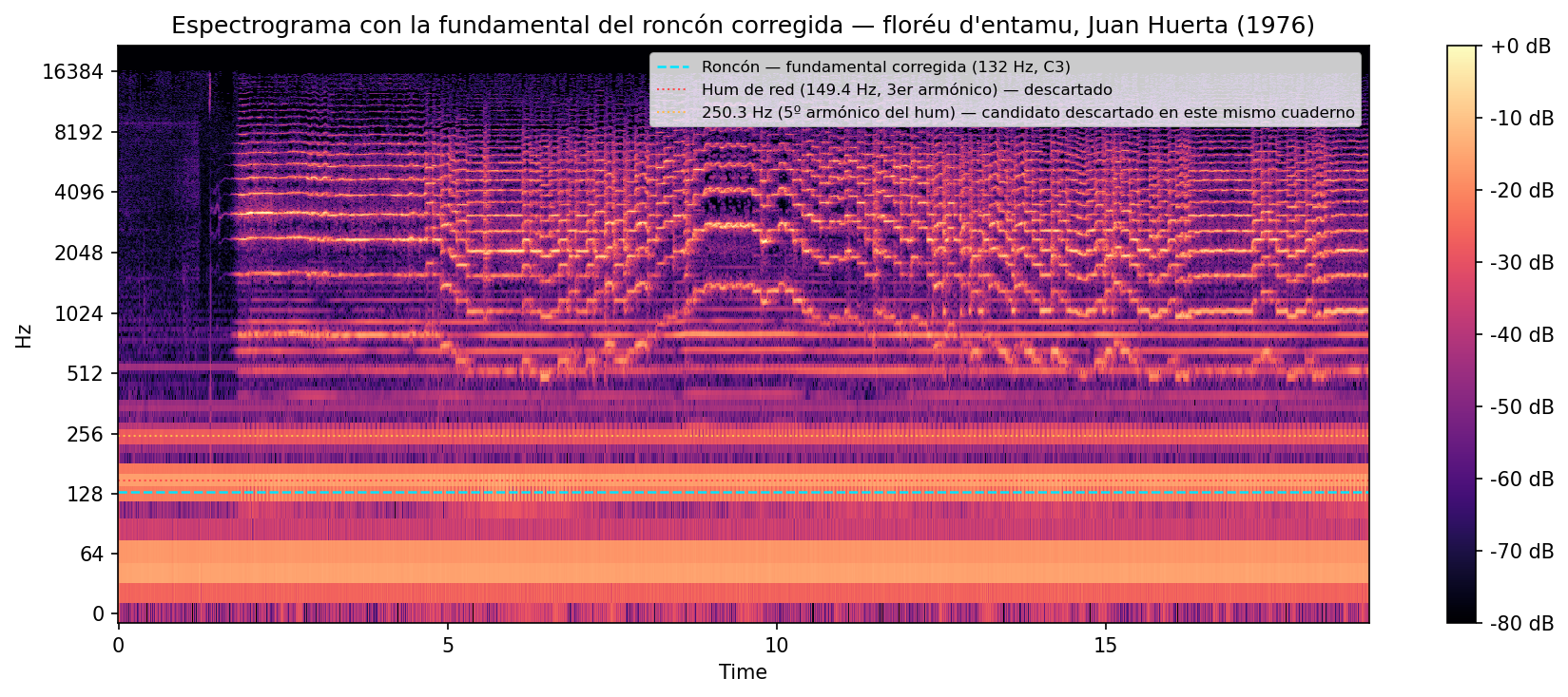
The roncón marked on the spectrogram: its main note, at 132.0 Hz (C3), holds as a constant horizontal band throughout the whole piece — also marked are the candidates discarded as spectral leakage from the mains hum.
The piece as it is: drone and melody mixed together
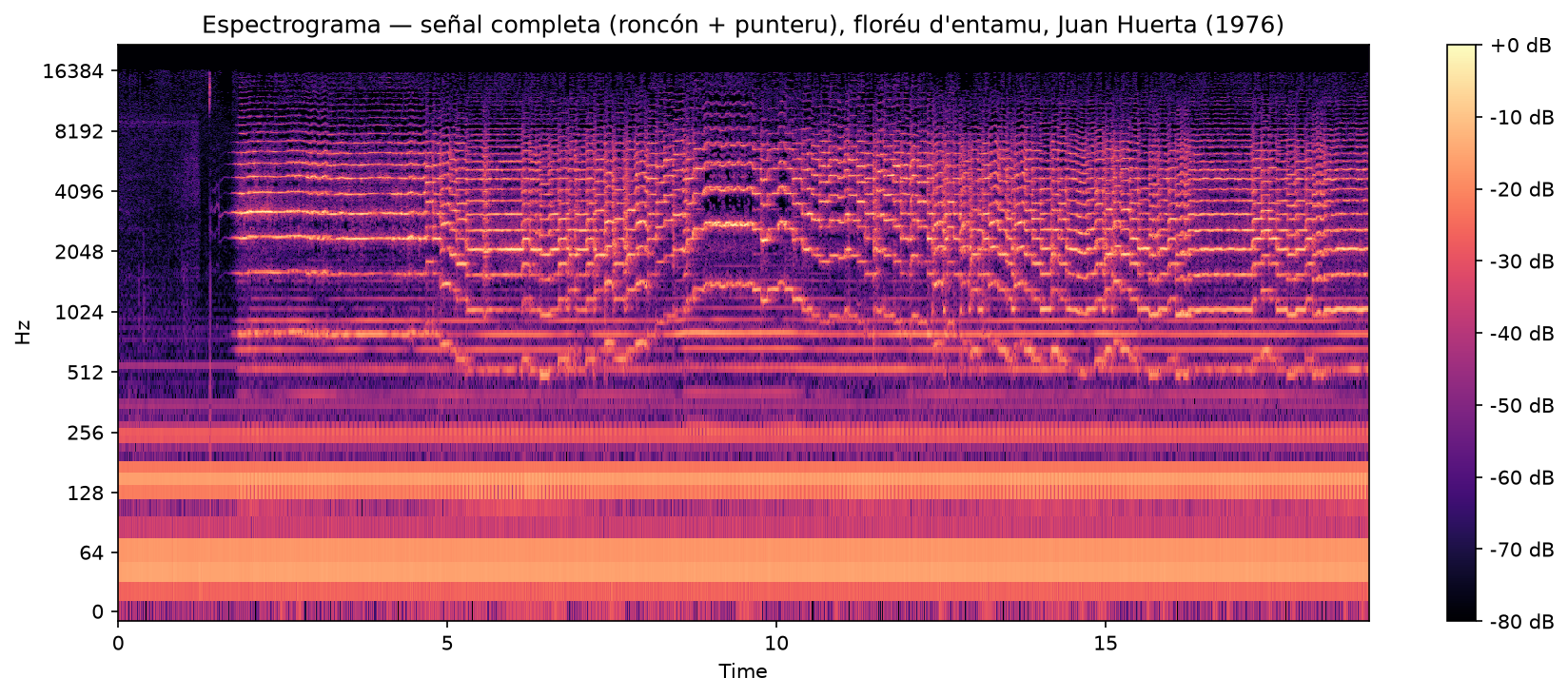
Before touching any of the audio, I analyzed the complete recording exactly as it arrived, with two different tools.
The first looks for onsets: the exact instant each note begins, the “attack” of the sound. It’s the first thing any system that wants to transcribe a piece into a score needs: knowing when something happens. Over the 19 seconds of this recording, the algorithm detects 127 onsets — nearly 7 new notes per second, a dense rhythm typical of the Asturian bagpipe.
The second task is pitch-tracking: figuring out, instant by instant, exactly which note is being played. For this I use a method called pYIN: an algorithm that, in each fraction of a second, calculates the most probable frequency sounding and how confident it is about it — it doesn’t guess, it measures — limited to the actual note range a punteru can play. The result: it detects a clear pitch in 92.7% of the instants analyzed — essentially across the whole fragment, failing only about 1 in every 13 instants.
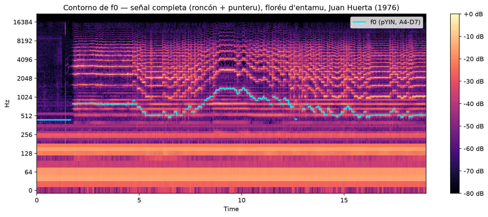
What does that line have to do with the actual piece? In my classes I teach the floréu d’entamu with a three-part scheme — opening, body and closing — each with its reference notes:
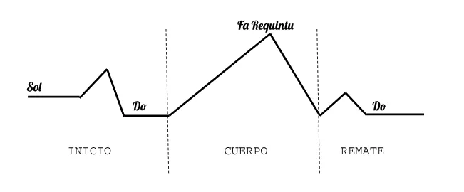
Comparing the detected f0 line against this diagram, what the algorithm detects matches the three parts, though in the opening the real shape is more contained than the “textbook” diagram’s:
- The peak of the body matches precisely. The highest frequency of the whole fragment — 1437.8 Hz, note F6 — appears at second 10.08, right in the middle of the body. It’s exactly the note the diagram marks as the climax: the Fa Requintu.
- The closing matches too. In the last three seconds, C (C5) is, by far, the note that appears most: 167 of about 238 instants analyzed. The diagram closes the piece on C, and that’s exactly what the algorithm measures.
- The opening matches, but with a shorter rise than the diagram’s. The real line rises to A4 (A) — not to a high C, as more expansive flourishes would, in the style of José Remis Ovalle (one of the masters who founded a school of playing in Asturies, with a style so recognizable that many pipers imitated it) — and from there descends to settle on C (C5) from second 5.3 onward. It’s the same underlying shape the diagram draws — rise and return to C — but with a shorter leap: a personal stylistic choice, not a flaw in the diagram or the algorithm.
That nuance in the opening is, in fact, the most interesting part of the comparison: the diagram gives the general shape of the phrase — where it rises, where it falls, where it closes — but doesn’t fix the exact amplitude of each flourish, which varies by player and performance. Comparing automatic analysis against the “textbook” form of a piece is a real way to see, note by note, how a specific performance moves within that form.
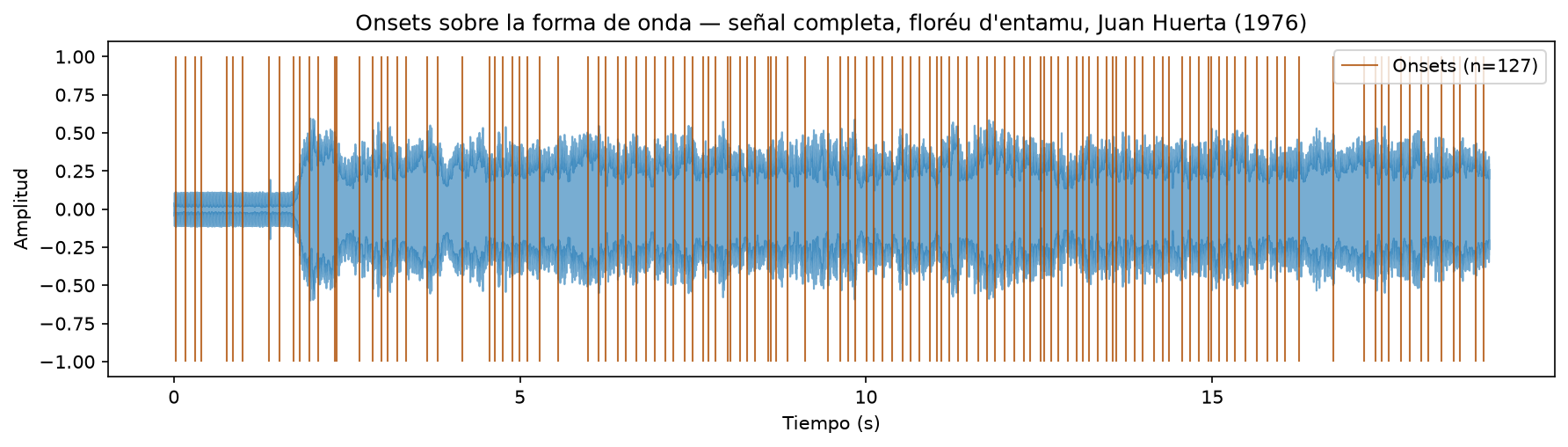
These three results are the starting line: what the analysis gives without touching any of the audio. The next question is whether removing the roncón before analyzing improves on this.
Can the drone be separated from the performance?
To try to get the roncón out of the way, I tested the standard technique used for cases like this: HPSS (Harmonic-Percussive Source Separation). Picture it as a sieve — a colander with a mesh that lets some things through and holds others back — that strains the sound into two trays: into one fall the “percussive” sounds — like a bass drum or a click, which start suddenly and die out fast — and into the other fall the “sustained” sounds — harmonic, like a piano or violin note held over time. The roncón is, by definition, a purely sustained sound: it doesn’t attack suddenly, it sounds the same the whole time. The bet was a reasonable one: if the sieve separates sustained from percussive well, the roncón should fall entirely into one of the two trays, leaving the other cleaner.
The result is that the sieve doesn’t work here, and it’s worth explaining why. HPSS was designed for cases like separating a piano from a drum kit — there, a real boundary exists between “sounds sudden” and “sounds sustained.” But in the Asturian bagpipe, both the roncón and the punteru melody are sustained sounds — neither is percussive, neither “attacks suddenly” and dies out. To the sieve, roncón and melody are the same grain of sound: both fall into the same tray, with no way to tell them apart through this route.
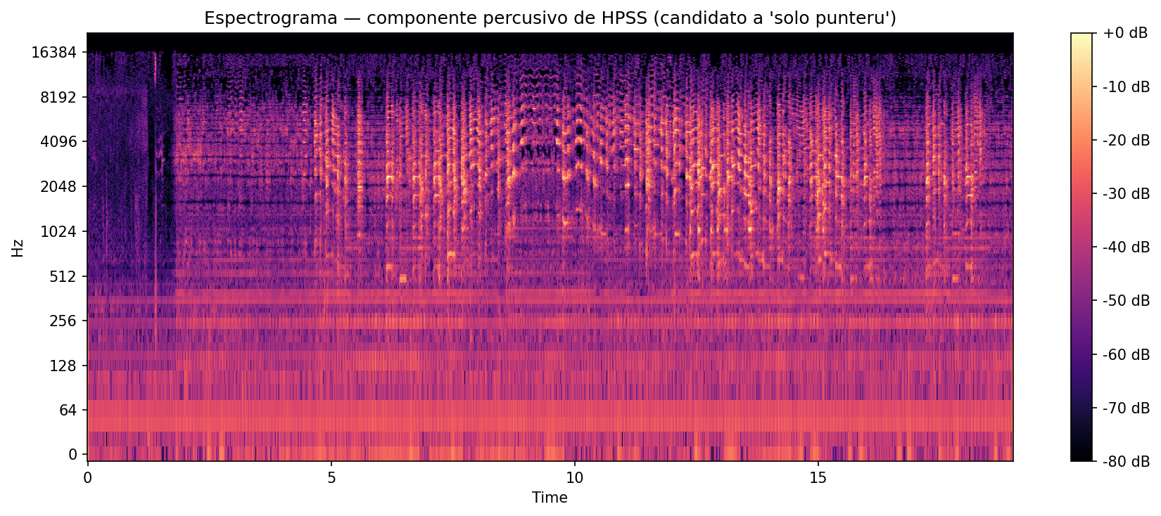
The numbers confirm it. Measuring again with RMS — the same “how loud on average” from the previous section — the “sustained” tray keeps 92.5% of the sound’s total energy — the roncón goes there almost entirely, dragging a good chunk of the melody along with it. The “percussive” tray barely retains 19.0%. And if I look specifically at how much of the roncón’s energy ends up in each tray, the difference is still enormous: the sustained tray holds 77 times more roncón energy than the percussive tray — using the correct frequency band (132 Hz, now without the mains hum contamination), rather than the inflated band from the earlier version. At first glance this might look like a very clean separation of the roncón — but it isn’t: what actually happened is that the sieve pushed almost everything sustained, roncón and melody together, to the same side.
As a simpler comparison, I also tried a notch filter: instead of a sieve that classifies, it’s a scalpel that surgically cuts out a single exact frequency — in this case, the roncón’s 132 Hz — leaving everything else intact. The result of this comparison is in the next section.
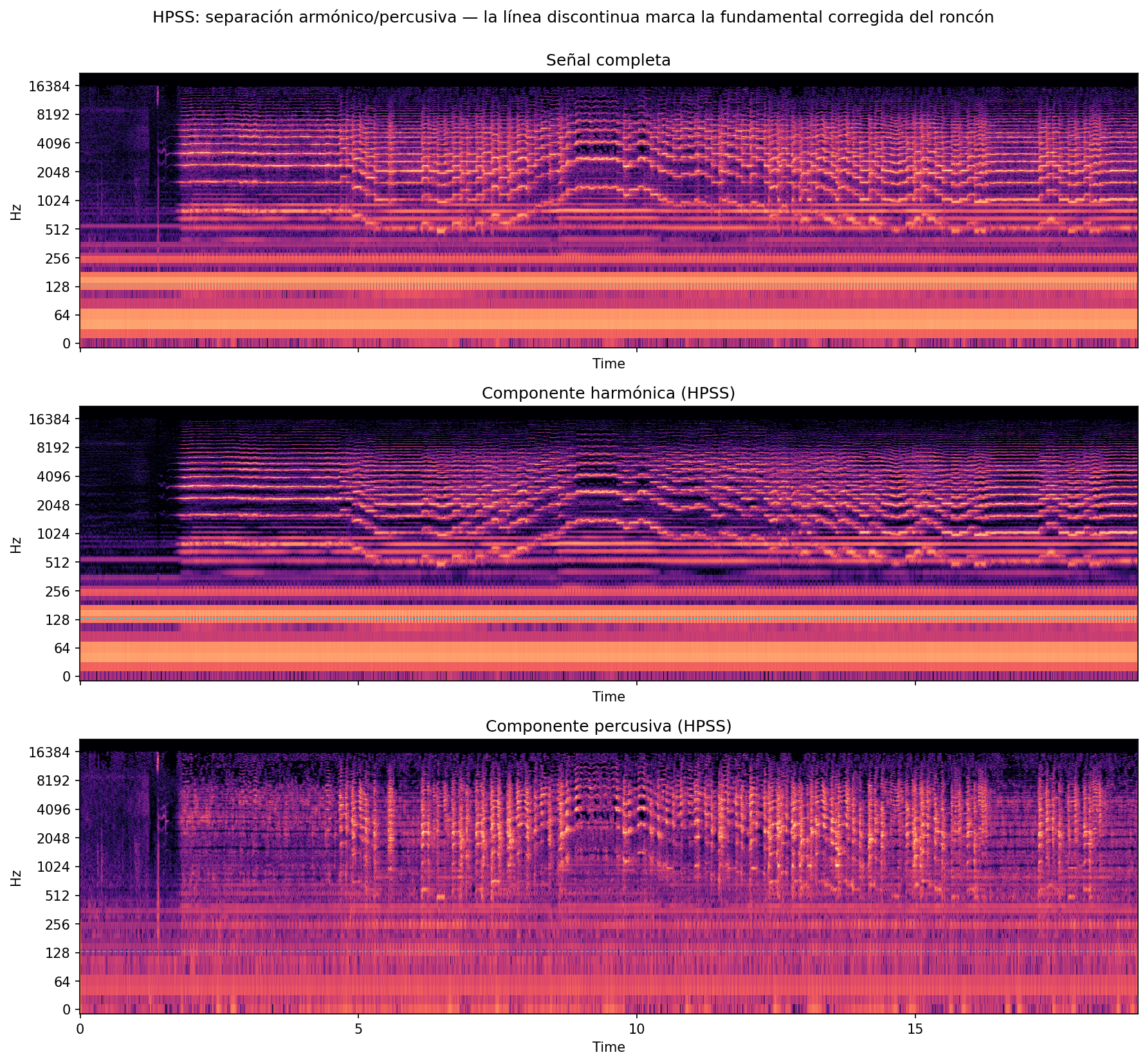
HPSS comparison: full signal, “sustained” tray (keeps 92.5% of the sound, including the roncón) and “percussive” tray (only 19.0%).
What this result actually says
This isn’t just “the technique failed” — it’s a finding about what “separating the roncón” even means for this particular instrument. The HPSS sieve can’t tell apart “sustained roncón” from “sustained punteru note,” because to it, both are exactly the same kind of sound. The next section’s result — pitch-tracking gets much worse, onsets barely change — confirms that separating by “sustained versus sudden” is the wrong tool for this case, not that separating roncón and melody is impossible with any technique. It’s a real, useful finding: it explains precisely why the Asturian bagpipe — a continuous drone and a melody, both sustained, sounding at once — is a genuinely hard case for this kind of automatic analysis, beyond just “it’s an old, noisy recording.”
The analysis after separating
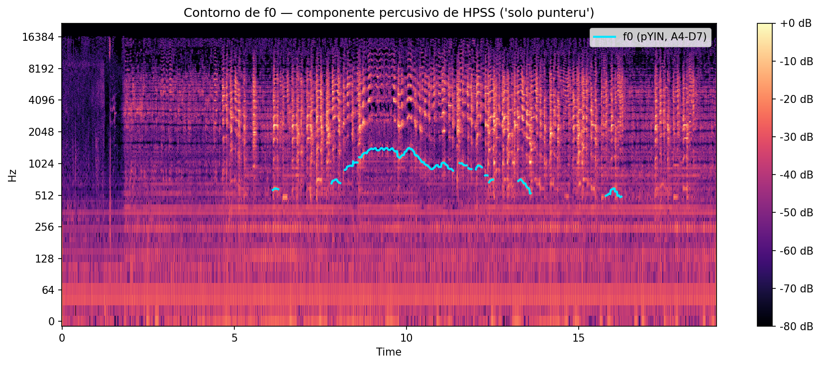
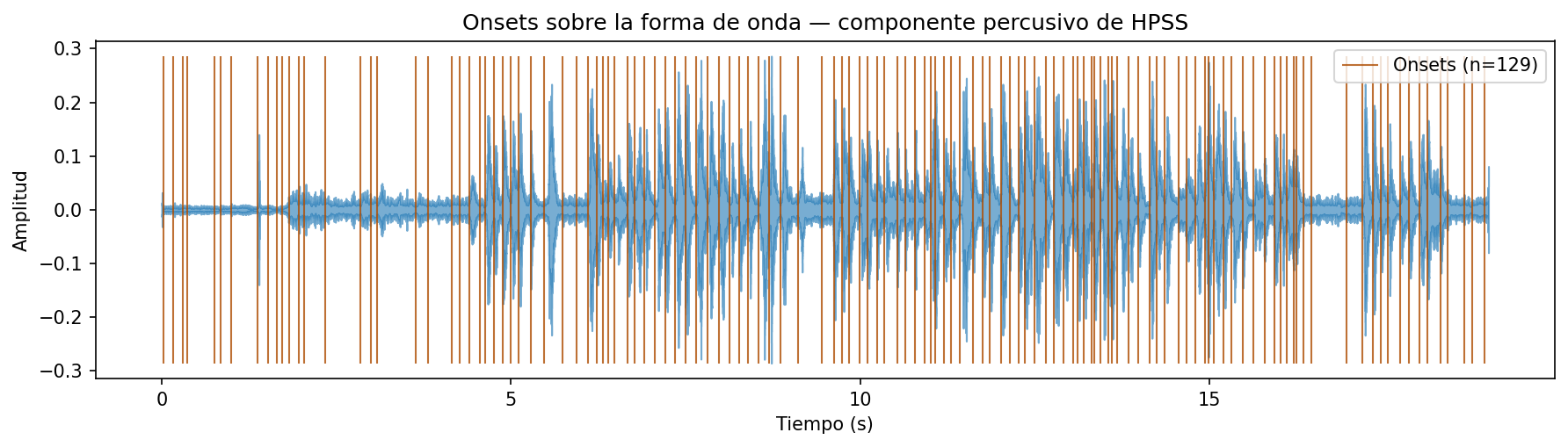
With HPSS’s “percussive” tray — the result that, in theory, should resemble “melody only” the most — I repeated the two earlier analyses. Pitch-tracking collapses: from detecting a note in 92.7% of the instants it drops to just 26.7% — practically 1 in every 4 instants, when before it got nearly all of them right. That’s a huge loss of useful information. Onsets, by contrast, barely move: 129 versus the 127 of the full signal, a difference small enough that it doesn’t count as a real improvement.
The notch filter — the surgical scalpel that only cuts out the roncón’s exact note — behaves just as you’d expect from a much more precise, less aggressive intervention: pitch-tracking stays practically the same, at 92.7%, the same value as with the full signal. It changes so little because it only removes the exact frequency of the roncón, leaving its harmonic echoes intact — which, unfortunately, fall right in the same frequency range where the punteru melody moves, so they don’t help clean it up much either — and onsets stay exactly the same, at 127.
Conclusions
The question that motivated this experiment was direct: does this preprocessing help analyze the Asturian bagpipe better? The verified answer is no. Note attacks barely change (127 versus 129, practically the same) and melody tracking gets much worse (from 92.7% down to 26.7% of instants with a detected note). The HPSS sieve fails to isolate the punteru: it doesn’t separate the roncón well, and in the process it takes a good chunk of the melody itself down with it.
What can be said with confidence: the difficulty of analyzing the Asturian bagpipe with these tools isn’t just a matter of “it’s an old recording.” It’s something intrinsic to the instrument — a continuous drone and a melody sounding at once, both sustained, with no “sudden versus sustained” boundary that a sieve like HPSS can use to tell them apart. Effectively separating the two would probably require a different technique — but I didn’t test any, and I’d rather leave that as an open question than promise a solution I haven’t verified.
The whole analysis — spectrograms, HPSS, pYIN, onsets, the exact figures in this article — is in the notebook I ran to write it, with the outputs already computed. Download it along with the audio fragment itself and repeat the experiment yourself, note by note.
Analysis notebook (Jupyter)
Python + librosa. Includes the calculation of this article's figures and the already-run figures.
References
- McFee, B., Raffel, C., Liang, D., Ellis, D. P. W., McVicar, M., Battenberg, E., & Nieto, O. (2015). librosa: Audio and Music Signal Analysis in Python. Proceedings of the 14th Python in Science Conference, 18–24.
- librosa official documentation — source of
onset_detect,pyinandeffects.hpss, used in this analysis. - Mauch, M., & Dixon, S. (2014). pYIN: A fundamental frequency estimator using probabilistic threshold distributions. 2014 IEEE International Conference on Acoustics, Speech and Signal Processing (ICASSP), 659–663.
- Celso Peyroux Sound Archive, Oviedo — cassette no. 1, April 1976, performer Juan Huerta (La Torre, Teverga). Primary source of the recording analyzed.
- Header photograph: family archive of Juan Huerta, lent for Tever Díaz García’s research on the folk musicians of Proaza and Teverga.
- All the figures in this article were independently reproduced by running the notebook twice, with identical results.