
Tutorial · DIY Lab
How to compute a spectrogram with librosa
A step-by-step tutorial, with a downloadable notebook, on going from real audio to its spectrogram with librosa: STFT, decibels, and reading harmonic bands.
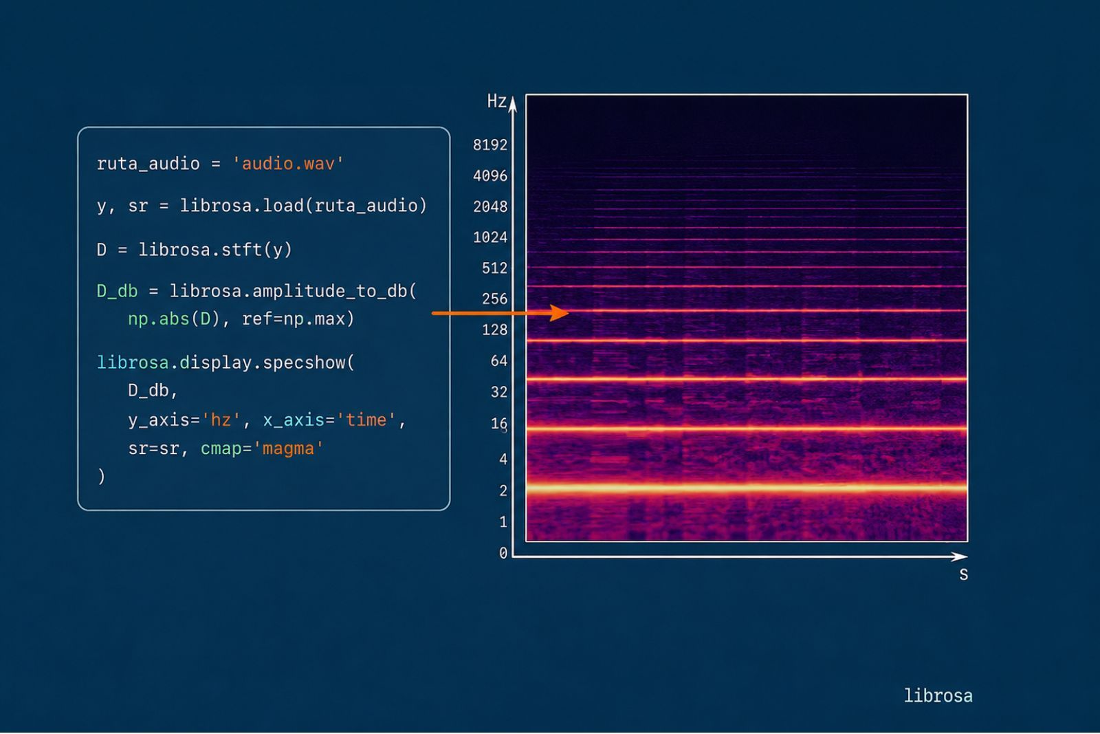
librosa is the reference Python library for working with audio: it computes spectrograms, extracts features, and gives you direct access to the Fourier transform without you having to implement it yourself. This tutorial goes from theory to practice: we load a real audio clip, compute its spectrogram, and learn to read it. At the end you’ll have a downloadable Jupyter notebook with all the code, ready to run on your own audio.
What we’re going to build
We start from a real audio excerpt —a fragment of Fayendo (2021), a track from the EP Suañu de Gaita, my own recording of Asturian bagpipe— and walk through the full path to its spectrogram:
- Load the audio with
librosa.load. - Compute its short-time Fourier transform (STFT).
- Convert that transform into a readable spectrogram, in decibels.
- Plot it and learn to read what it shows.
All the code in this tutorial also lives in a Jupyter notebook you can download and run with your own audio.
Installation
pip install librosa numpy matplotliblibrosa brings numpy as a dependency, but matplotlib has to be installed
separately for plotting. With those three libraries installed, you can
reproduce everything that follows.
1. Load the audio
import librosa
import librosa.display
import numpy as np
import matplotlib.pyplot as plt

y, sr = librosa.load("tever-extracto.mp3")

print(f"Sample rate: {sr} Hz")
print(f"Duration: {librosa.get_duration(y=y, sr=sr):.1f} s")
librosa.load decodes the file and returns two things: y, a numpy array
with the waveform, and sr (sample rate), the sampling frequency. By
default, librosa resamples to 22050 Hz —enough for the range of interest in
music analysis, and lighter to process than the 44100 Hz of a CD.
2. The short-time Fourier transform (STFT)
The waveform doesn’t easily tell you which notes are sounding: it’s the time-domain representation, an air-pressure value per instant. To see which frequencies it contains you have to move to the frequency domain, and not all at once over the whole audio, but in short windows that slide over time. That’s the STFT (Short-Time Fourier Transform): many small Fourier transforms, one per window, stacked one after another.
D = librosa.stft(y, n_fft=2048, hop_length=512)Two parameters decide the resolution of the analysis:
| Parameter | What it controls |
|---|---|
n_fft | The size of each analysis window, in samples. 2048 is a common value: enough frequency resolution without losing too much time resolution. |
hop_length | How much the window shifts between successive computations. With overlap (hop_length smaller than n_fft), the result comes out smoother. |
D is a matrix of complex numbers: each column is a time window, each
row a frequency, and the value combines magnitude (how much energy there is)
and phase.
3. From magnitude to decibels
For the spectrogram you only need the magnitude, not the phase. And since the human ear perceives intensity logarithmically, it’s converted to decibels:
S_db = librosa.amplitude_to_db(np.abs(D), ref=np.max)That way, small differences in low-energy areas stand out as clearly as large ones in high-energy areas —on a linear scale, they’d get flattened out.
4. Plot the spectrogram
fig, ax = plt.subplots(figsize=(12, 5))
img = librosa.display.specshow(
    S_db, sr=sr, hop_length=512,
    x_axis="time", y_axis="log", ax=ax, cmap="magma",
)
ax.set(title="Spectrogram (STFT, logarithmic scale)")
fig.colorbar(img, ax=ax, format="%+2.0f dB")
plt.show()
specshow reads the time and frequency axes directly from sr and
hop_length, so you don’t have to compute them by hand. The logarithmic Y
axis (y_axis="log") is standard in music: it better reflects how notes are
distributed across the audible range than a linear scale would.
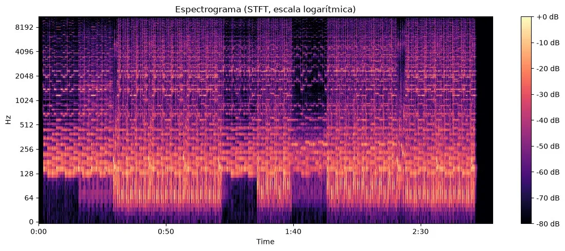
Spectrogram of an excerpt of Fayendo, computed with the code in this tutorial. The horizontal bands are the harmonics of each note; the vertical gaps, silences between phrases.
How to read the result
In the spectrogram above you can see horizontal bands rising and falling together: they are the fundamental frequency of each note and its harmonics —integer multiples of that frequency—. That pattern of parallel bands, and how the energy is distributed among them, is one of the signals a automatic music transcription system uses to decide which note is being played. The vertical gaps of silence between bands correspond to the breaths between phrases —a feature typical of phrasing on continuous-air wind instruments, like the bagpipe.
Next steps
This tutorial stops at the spectrogram as an image. The downloadable notebook points to three directions to keep going:
- Chromagram (
librosa.feature.chroma_stft): groups the energy into the 12 pitch classes (C, C#, D…), useful for detecting chords or key. - MFCCs (
librosa.feature.mfcc): a compact representation of timbre, widely used in instrument and genre classification. - Onset detection (
librosa.onset.onset_detect): finding the exact instant each note starts, a first step toward real automatic transcription.
The notebook
All the code from this tutorial —loading, transforming, plotting, and the
commented next steps— is in a
downloadable Jupyter notebook,
along with the fragment of
Fayendo used as an example. Open it with
jupyter notebook or jupyter lab, or upload it to
Google Colab if you don’t want to
install anything locally. If you’ve never used one before,
What a Jupyter notebook is explains where to
start.
References
The references this article draws on, and where to read further:
- McFee, B., Raffel, C., Liang, D., Ellis, D. P. W., McVicar, M., Battenberg, E., & Nieto, O. (2015). librosa: Audio and Music Signal Analysis in Python. Proceedings of the 14th Python in Science Conference, 18–24.
- librosa official documentation.
- Müller, M. (2015). Fundamentals of Music Processing: Audio, Analysis, Algorithms, Applications (ch. 2 and 3). Springer.